Which sandpile matches the brain?
In 2003 John Beggs and Dietmar Plenz recorded bursts of electrical activity in slices of rat cortex. Burst sizes followed a power law with exponent 1.50. The textbook story for laws like that is a sandpile. I dropped 14 million grains on simulated sandpiles to find out which kind of sandpile actually gives 1.50.
Synthetic simulation. No patient data, uploads or recorded inputs.
The static simulation record is shown. Interactive controls are preparing; reload if they remain unavailable.
Drop some sand
Each cell holds up to three grains. A cell that reaches four topples and passes one grain to each neighbour. Grains pushed off the edge are gone. One dropped grain can do nothing, or it can set off a chain that crosses the board. That chain is an avalanche, and its size is the number of topplings.
Click or hold on the board to pour grains in one spot.
The board starts paused after 30,000 pre-run grain drops. Enable JavaScript to draw its log-log avalanche histogram and fitted power-law line.
Avalanche sizes on this board, both axes logarithmic. The line is a maximum-likelihood power-law fit over sizes 10 to 1,000. A 64 × 64 board gives a rough number, but switch the wiring and the slope still moves. The board starts with 30,000 avalanches already run, so the chart has data from the first frame.
Only random wiring lands on 1.50
The exponent τ in P(s) ∝ s−τ says how fast big avalanches get rare. Fitted over avalanche sizes 30 to 3,000 on the largest system of each kind, a 2D grid gives 1.12, a 3D grid gives 1.34, and random wiring gives 1.49. Cortex gave 1.50 ± 0.008.
The difference comes from wiring. When grains go to random cells, an avalanche almost never runs back into cells it already disturbed. It then behaves like a branching process, where each toppling sets off a random number of new ones, one on average. A critical branching process has exponent exactly 3/2. On a grid an avalanche keeps crashing into its own territory, and that changes the statistics. Above four dimensions a grid stops mattering and every sandpile gives 3/2, which is why the number climbs from 2D to 3D.
Beggs and Plenz made the same comparison. They measured a branching ratio near 1 and read their 1.50 as a critical branching process. So the brain's number fits a critical network whose connections are not limited to near neighbours. A sandpile on a flat sheet gives a smaller number.
None of this is new physics. The link between mean-field sandpiles, branching processes and 3/2 is in the textbooks. I wanted to see it fall out of a simulation I had checked myself, and the checks turned up one thing I did not expect, further down.
Where each sandpile lands
The fitted exponents are 1.49 for random wiring, 1.34 for a 3D grid and 1.12 for a 2D grid. The table provides the complete static record.
Dots are maximum-likelihood fits over sizes 30 to 3,000. The pale bar behind each dot shows how far the local slope wanders inside that range. Rings mark the value each model reaches on an infinite system: 3/2 for random wiring, 4/3 for the 3D grid, which was proved in May 2026, and about 1.29 for the 2D grid from finite-size scaling.
| Model | Fitted τ | Local slope | Infinite system | Grain drops |
|---|---|---|---|---|
| Cortexrat cortex slices, Beggs and Plenz 2003 | 1.50 ± 0.008 | critical branching | ||
| Random wiring10 million sites | 1.485 ± 0.004 | 1.48 to 1.51 | 3/2 | 1,000,000 |
| 3D grid96 × 96 × 96 | 1.338 ± 0.002 | 1.30 to 1.37 | 4/3 | 2,000,000 |
| 2D grid512 × 512 | 1.121 ± 0.002 | 1.08 to 1.13 | about 1.29 | 1,000,000 |
Slope at every scale
A power law is a straight line on log-log axes, and the exponent is its slope. One fitted number can hide a slope that drifts, so I also fitted the slope in a one-decade window that slides along the size axis. A clean power law shows up as a flat line.
Random wiring stays within 0.03 of 1.5 from size 30 to 10,000. The 3D grid drifts up through 4/3. The grid curves shoot up at their right ends, where the system's finite size cuts off the largest avalanches. The random-wiring curve stops near 18,000 because bigger avalanches are too few to fit.
The static table gives local fitted slopes across avalanche sizes. Enable JavaScript for the keyboard-readable local-slope and distribution views.
Local exponent from maximum-likelihood fits in one-decade windows that slide along the size axis. Lines leave the top of the frame at each system's finite-size cutoff. The horizontal line is the cortex value.
Show the numbers
| Avalanche size | 2D grid | 3D grid | Random wiring |
|---|---|---|---|
| 3 | 1.009 ± 0.003 | 1.171 ± 0.002 | 1.335 ± 0.003 |
| 10 | 1.039 ± 0.004 | 1.271 ± 0.003 | 1.451 ± 0.005 |
| 32 | 1.081 ± 0.005 | 1.298 ± 0.004 | 1.486 ± 0.007 |
| 100 | 1.110 ± 0.005 | 1.322 ± 0.005 | 1.476 ± 0.009 |
| 316 | 1.128 ± 0.005 | 1.342 ± 0.006 | 1.493 ± 0.012 |
| 1,000 | 1.121 ± 0.006 | 1.366 ± 0.008 | 1.494 ± 0.016 |
| 3,162 | 1.121 ± 0.006 | 1.399 ± 0.010 | 1.492 ± 0.022 |
| 10,000 | 1.098 ± 0.007 | 1.499 ± 0.013 | 1.505 ± 0.029 |
| 31,623 | 1.118 ± 0.007 | 1.642 ± 0.018 | |
| 100,000 | 1.394 ± 0.008 | ||
| 316,228 | 1.733 ± 0.012 | ||
| 1,000,000 | 2.254 ± 0.022 |
The 2D grid looks clean and is wrong
This is the part I did not expect. On the 512 × 512 grid the local slope stays between 1.08 and 1.13 from size 30 to 30,000, almost three decades. That looks like a textbook power law. It is not the exponent of an infinite grid.
Bigger grids give bigger fitted exponents, and slowly. Each doubling of the grid adds about 0.015. Lübeck and Usadel saw the same drift on grids up to 4,096 wide in 1997. Extrapolating my three grids their way gives 1.22, close to the 1.25 they got by the same method, and their better method gives 1.29. Anyone fitting a 2D sandpile directly would report a number that is too low, and a flat-looking slope plot would not warn them.
| Grid | Fitted τ, sizes 30 to 3,000 | Local slope range |
|---|---|---|
| 128 × 128 | 1.091 | 1.05 to 1.12 |
| 256 × 256 | 1.105 | 1.07 to 1.11 |
| 512 × 512 | 1.121 | 1.08 to 1.13 |
| Infinite grid, Lübeck and Usadel 1997 | 1.293 ± 0.009 |
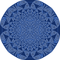
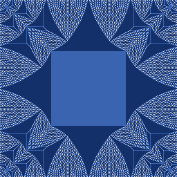
The same rule draws pictures
Sandpiles also have a mathematical side that has nothing to do with brains, and I could not resist it. Both pictures use the board's colours, from pale for empty cells to dark for three grains.
How I know the simulator is right
A simulation that draws a nice power law proves nothing by itself. Before trusting any exponent I ran these checks, and all of them passed:
- Exact mean size. Dhar showed in 1990 that the expected number of topplings follows from the inverse of the toppling matrix. I computed that number exactly for every system, and all 8 runs match it within 0.2%. Grain conservation pins the long-run mean, so this tests the toppling rule and the edges, not the shape of the distribution.
- Order does not matter. Three different toppling orders give identical final piles and identical per-cell toppling counts. That licenses the shortcut of firing a cell several times at once.
- No grain goes missing. Every run checks that grains dropped equal grains on the board plus grains lost, to the grain.
- The grid reached its steady state. The 512 × 512 grid settles at 2.123 grains per cell. The infinite-grid value is 17/8 = 2.125, and the open edges pull a finite grid slightly lower.
- The fitter recovers known answers. On synthetic power laws with exponents 1.2 and 1.5 it returns 1.198 to 1.203 and 1.495 to 1.500.
- Runs had settled. Fits on the first and second halves of every run agree within 0.006.
- The pictures are what they claim. The identity satisfies e + e = e exactly. The single-cell pile keeps all 100,000 grains and exact eightfold symmetry.
Mean avalanche size, simulated against exact
| Run | Exact | Simulated | Difference |
|---|---|---|---|
| 2D grid, L = 128 | 593.89 | 593.38 ± 2.12 | −0.086% |
| 2D grid, L = 256 | 2339.30 | 2339.22 ± 10.74 | −0.003% |
| 2D grid, L = 512 | 9284.93 | 9285.40 ± 77.60 | +0.005% |
| 3D grid, L = 32 | 23.96 | 23.95 ± 0.15 | −0.042% |
| 3D grid, L = 64 | 89.14 | 89.13 ± 0.82 | −0.011% |
| 3D grid, L = 96 | 195.63 | 195.73 ± 2.19 | +0.051% |
| Random wiring, N = 1,000,000 | 250.00 | 249.91 ± 6.03 | −0.036% |
| Random wiring, N = 10,000,000 | 2500.00 | 2495.74 ± 149.40 | −0.170% |
Sources
- Bak, Tang, Wiesenfeld. Self-organized criticality: an explanation of 1/f noise. Phys. Rev. Lett. 59, 381, 1987.
- Dhar. Self-organized critical state of sandpile automaton models. Phys. Rev. Lett. 64, 1613, 1990.
- Beggs, Plenz. Neuronal avalanches in neocortical circuits. J. Neurosci. 23, 11167, 2003.
- Lübeck, Usadel. Numerical determination of the avalanche exponents of the Bak-Tang-Wiesenfeld model. Phys. Rev. E 55, 4095, 1997.
- Lübeck, Usadel. Bak-Tang-Wiesenfeld sandpile model around the upper critical dimension. Phys. Rev. E 56, 5138, 1997.
- Li, Liu, Shiraishi. Tail exponents of the three-dimensional uniform spanning tree and Abelian sandpile. arXiv:2605.19419, May 2026.
- Levine, Pegden, Smart. Apollonian structure in the Abelian sandpile. Geom. Funct. Anal. 26, 306, 2016.
- Levine, Pegden, Smart. The Apollonian structure of integer superharmonic matrices. Ann. Math. 186, 1, 2017.
Experiment updated 2026-10-01. Part of dhupbh.com. IBM Plex, SIL Open Font License. Board activity stays in this browser and is not recorded by page analytics.